This overview of the groundwater surface is a synthetic calculation result, and hence an intermediate result. The representation and interpretation of this intermediate result is moreover an important plausibility check for the determination of the depth to the water table, since its integration with the altitude model incorporates new, independent information into the model. Any uncertainties in this result may then stem from implausibilities in one or the other of the two independent information sources.
By the inclusion of the lower edges of the aquitard layers, the areas in which the confined potentiometric surface is located under a thick marly till cover at a great depth are shown. At the same time, the “jumps” of the potentiometric surface are also recognizable at the edges of the confined and unconfined groundwater areas.
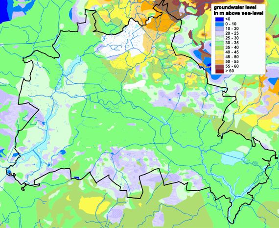
On the Barnim Plateau, the deep areas are located particularly in the northeast (Rosenthal) and along the southern edge of the ground-moraine plate (Lichtenberg). Here, the confined groundwater surface lies near to, or, locally, even deeper than sea level. These are also mostly areas in which there is no main aquifer, or only one of isolated expanse. However, within the confined areas in Frohnau, the groundwater surface dips to only about 15 meters above sea level.
The southern part of the Teltow Plateau (Marienfelde, Buckow) is characterized by maximum depths of the groundwater surface of about 10 meters above sea level. Very deep-lying areas are also recognizable in the area of the plateau sands of the Teltow Plateau east of the Havel; locally they drop roughly to sea level here. This is also the case west of the Havel; mostly however, the groundwater surface in the confined areas here is between 10 and 25 meters above sea level.
The highest levels of the groundwater are found at altitudes between 55 and 60 meters above sea level in the north-eastern, unconfined area of the Panke Valley in Buch, on the Brandenburg state line. Outside Berlin, the groundwater surface on the Barnim Plateau rises to even higher than 60 metres above sea level in some places, but also shows very great fluctuations over small areas (e.g. at the city limits at Ahrensfelde). The groundwater surface in the northwest of Berlin within the glacial spillway is at a relatively homogeneous standard; however, around Marwitz, in the confined area, it drops considerably again. South of Berlin, in the Teltow area, where varying confinement conditions prevail, it is generally above 35 metres, and in some places even above 40 metres above sea level.
The unconfined area of the Panke Valley contrasts sharply with the surrounding confined areas, with altitudes of the groundwater surface of mostly 40 to 50 meter above sea level. The largest “jump heights” in groundwater surface are also recognizable at the edges of the Panke valley, locally reaching up to 40 meters in vertical difference over a horizontal distance of only a few hundred meters (e.g. on the eastern edge, at the level of Blankenburg). Thanks to the initially separate calculation of depths to groundwater which were then aggregated, no mutual effect due to the regionalization process – which does not exist in nature – occurred here.
In the glacial spillway, the groundwater surface reflects the groundwater contour lines. It shows a continuous drop of the groundwater surface in the direction of flow for both the significant tributaries to the main aquifer, the Spree and the Havel, i.e., from east to west and from north to south, respectively. This reflects the hydraulic contact between the surface and the groundwater, which exists everywhere in this area.
Subsequently, a difference model was calculated from the Model of the Groundwater Surface and the Terrain Elevation Model. The grid width there was 5 meters.
In addition to the 5 m model, other models with larger grid distances (10, 25, 50 and 100 m) were calculated, which, depending on the display scale, are represented in the GIS. For the PDF map, a grid interval of 25 m was chosen.
The depths to groundwater were broken down into 14 depth classifications and published as a map of stratum levels. In order to differentiate depths to groundwater in the range of up to 4 meters, especially in areas important for vegetation, a detailed classification was chosen there.
For smaller areas, it is possible to obtain more precise results with the digitalized data available, using smaller grid widths to interpolate the data. The classification boundaries between the categories of depths to groundwater can also be chosen arbitrarily, and are also available with discrete information in the calculated data base.
The exactness of the data of the Depth to Groundwater Model is directly dependent on the quality of the Terrain Elevations Model. Therefore, the levels of precision indicated for the elevation models are generally also valid for the depth to groundwater map. For the DTM25 used on Brandenburg territory, the level of precision is +/- 2 m; for the DTM5 used on Berlin territory, it is +/- 0.5 m or better.
The following points should be considered, to avoid false interpretations:
- Because of the state of the data, the Terrain Elevations Model will show some inaccuracies. This involves on the one hand areas in the state of Brandenburg which are not yet covered by the DTM5. On the other, in the areas covered by the DTM5 data, some methodological errors, such as misinterpretation of the results of the laser scan method in cases where glass roofs and solar panels are present, leading in some cases to false terrain elevations and hence to depressions with slight depths to groundwater which do not in fact exist. Such areas occur e.g. in the densely-inhabited inner city area, but they are rare and of limited extent.
- In areas where groundwater is located under thick, relatively impermeable, marly-till aquitard layers, and is thus usually confined, the depths to groundwater can be assumed to be more than 10 meters, and often even more than 20 meters. The lower edge of the aquitard is assumed to be the upper surface of the groundwater. Sandy interstratifications in and on these marly-till layers, within which near-surface or only seasonally present groundwater can also appear, are very limited spatially, and their sites can be localized only with great effort; they have therefore not been taken into account in the determination of depth to the water table. Particularly in confined areas with an only isolated quaternary main aquifer, near surface occurrence of groundwater is also common (e.g. at Tegel Creek).
- The upper surface of the groundwater is subject to strong fluctuations in areas near wells, depending on withdrawal quantities. For this reason, locally greater depths to groundwater can occur here. The sizes of these areas too cannot be portrayed in the scales used here.
- It is to be noted that not all wetland areas potentially valuable for the protection of biotopes and species can be gleaned from the Map of Depth to the Water Table (depth to groundwater less than 1.0 meter). This includes areas which, e.g., have no connection to groundwater and are watered by dammed water or periodic natural flooding (such as the Tiefwerder Meadows, or Tegel Creek).