Future Climatic Change and Thermal Load 2008

Methodology

Evaluation of thermal load situations can be carried out using various criteria. “The most frequently used is Fanger’s Comfort Equation (1972), and the Perceived Temperature (PT) calculated from it, by means of which the thermal effect complex is determined” (VDI 2008).

The urban bio-climate model UBIKLIM (Urban Bio-Climate Model) is a model method which builds upon those criteria. It was developed for practical application in urban planning by the Deutscher Wetterdienst (DWD), and has been applied in Berlin since 1996 to assess the thermal situation of a typical summer’s day (see SenSUT 1998).

The unusual methodological-technical feature of UBIKLIM was the development of a projection of the bio-climate for time periods subject to climatic change, i.e., over the next 30 – 70 years. Since no standardized methods yet exist for this purpose, the results presented here regarding the application of UBIKLIM in the context of climate projections should be considered as estimates of the future development of the climate. Based on climate projections, climate change scenarios which represent possible plausible developments of the climate in the future can be designed. They cannot, however, be treated as exact forecasts or even as weather forecasts (UBA; German only).

Input Quanta and Procedures at UBIKLIM

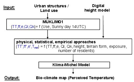
As input quanta, UBIKLIM needs not only a high-resolution height model, but also suitable land use information. For this purpose, the area under examination is subdivided into a finite number of sections with the same or similar uses. Built-up areas are further subdivided and clearly characterized according to degree of soil sealing, proportion of built-up areas, building height, number of buildings per unit of area, and proportion of green space. Using these input data, UBIKLIM calculates the meteorological quanta for the entire area under examination at a height of 1 m above ground on a cloudless, low-wind summer’s day, in several steps – primarily by using the 1-dimensional urban climate model MUKLIMO_1 – and then analyses the results pixel by pixel using the Klima-Michel Model (see flow chart, Fig. 5). The resolution of the resulting bio-climate map is 10 to 25 metres.

UBIKLIM permits ascertainment of local differences in the bio-climate. However, these results do not provide any reference to the regional climate, and thus do not provide the basis for absolute information.

Fig. 5: Schematic structure of the urban bio-climate model UBIKLIM (TT: air temperature; ff: wind speed; e: humidity; Ql: long-wave solar flux, Qk: short-wave solar flux; Tmrt: average radiant temperature of a human; values for 1 m above ground)

Advancement of UBIKLIM to a Comprehensive Urban Bio-Climate Model

Bio-climate maps that reference the regional bio-climate and local differentiation can be generated by linking the UBIKLIM results to regional bio-climate information, which disregards land use and which is hereinafter described as the “background load”. The urban bio-climate model is thus expanded to a combined urban bio-climate model, which consists of UBIKLIM, the bio-climatically prepared background information, and a statistical model equation which is used to combine the different scales.

To be representative of a broader surrounding area, the weather data, largely unaffected by land use, are gathered at synoptic stations according to the specifications of the World Meteorological Organization (WMO). They are thus suitable for obtaining the required background information. Certain stations that differ considerably from the specifications are excluded. Their readings are characteristic of the climate in the immediate surroundings of the station, such as Berlin-Alexanderplatz, the “city centre”.

The 30-year average number of days with thermal load is used to determine the background thermal load outside the urban area. A thermal load day is defined as a day on which the Perceived Temperature reaches or exceeds 32°C – high thermal load – at a minimum of three hourly measurements between 9 and 15 UTC (Coordinated Universal Time) over the course of the day. This definition was chosen because it generally includes the days on which heat warnings are issued, i.e., which are of high thermo-physiological relevance.

In order to ascertain the connection between the thermal conditions on a sunny summer day and the mean climatic conditions, various urban and use structures were imposed on the weather data gathered from the synoptic stations in Germany for the 1971 – 2000 period. In other words all measurements for temperature, humidity, wind, and solar radiation derived from cloud cover data were modified according to land use. The modification parameters for the various urban structures were determined from MUKLIMO_1 simulations.

All data were then analysed with the Klima-Michel Model, and examined for thermal load days. The following regression equation was then derived from the data set obtained:

WB = (r₁*WB_frei + r₂*dGT + r₃WB_frei *dGT + r₄*nn + r₅ br + r₆*lä + r_konst) (Equation 1)

WB Thermal load days at an arbitrary point in the city
WB_frei Background load
dGT Perceived Temperature at an arbitrary point in the city minus Perceived Temperature above open spaces outside the urban area (as per UBIKLIM)
nn Altitude above sea level
br Latitude
lä Longitude
r_i Regression coefficients

Since the UBIKLIM results refer to sunny days, the thermal load days that are not sunny must also be taken into account, in order to couple the model with the regional bio-climate model. The resulting equation thus consists of both a regression equation and a weighting function. A sunny day is defined as the average of the 6, 12 and 18 UTC hourly values for cloud cover (N) and wind speed in 10 m above ground (v). On a sunny day, N

Tab 4: Comparison of Perceived Temperature as calculated by UBIKLIM (GTUBIKLIM), with average Perceived Temperature values ascertained from measurements at five climate stations in Berlin, on twelve sunny summer days (GTStation), 1990-2000

Table 4 shows the Perceived Temperatures from the model, compared with the average measurements at selected climate stations in the city for twelve sunny days. Clearly, the differences between urban structures are shown fairly well. Both the measurements and the model calculations show that similar thermal conditions prevail at the three airports. The Perceived Temperatures are approx. 2.5 to 3.5°C higher at the two urban stations; in the model, the difference is approx. 4°C, and reflects very well the respective situations of these urban stations – on the one hand, the city centre (Alexanderplatz); on the other, detached family homes with gardens (Dahlem).

However, this comparison should not be overstated, since point-based values (station data) are compared to area mean values (model data). Since an interpretation precise down to the pixel is impossible according to model philosophy, the model temperatures have been taken as representative for the approximate area of the station, However, since the data of the climate stations are considered representative of the surroundings, and in addition reflect a mean of several days, the comparison is nevertheless considered quite valid.

In the next step, the relationship to regional climate conditions was established. This was necessary in order to combine UBIKLIM with the data of the regional climate models REMO and WettReg used for future projections.

Application of the Comprehensive Urban Bio-Climate Model UBIKLIM

For the combined urban bio-climate model, in addition to the UBIKLIM input parameters, values for the background load and the percentage of sunny days are also needed. In the case of Berlin, these can be obtained from the data from the Berlin-Schönefeld climate station. The annual mean value is 9.9 thermal load days for the 1971 – 2000 period, with 47% sunny days. The geographical data, summarized as the quantum “geo” (see Equation 2), are assumed to be constant, due to the relatively small area involved.

Map 04.12.1 (see Fig. 8) shows the distribution of the thermal load days as a result of the model application for the 1971 – 2000 period.

It provides absolute information which can be compared with evaluations obtained in the same manner, e.g. from other cities, or also simply with the background load of any area.

Similarly to the comparative representation of the Perceived Temperatures in Table 4, Table 5 compares the station evaluations of the frequency of thermal load days with the model values. Unfortunately, the readings for the Alexanderplatz station were far from sufficient to ascertain – or even estimate – a 30-year mean. The station and model values show a good level of agreement. All three airport stations show approximately the same load level, while seven thermal load days more per year are shown for the area of the Dahlem urban station.

Tab 5: Comparison of no. of thermal load days calculated as per UBIKLIM (WBUBIKLIM), with no. of thermal load days calculated from the data from four Berlin climate stations (WB Stations) (ref. period: 1971-2000)

Projection of the Bio-Climate to Periods of Climate Change

Global climate models grew out of weather prediction models, and have been used since about 1940 to arrive at an understanding of future climate development. A range of scenarios is provided which differ according to their initial assumptions on future basic conditions, particularly regarding the emission of greenhouse gases and aerosols, and depend on socio-economic and technological developments. This scenario-based approach implicitly indicates the great fuzziness of climate projection, which should not be forgotten, even if only one scenario (Scenario A1B of the IPCC’S SRES Emissions Scenarios) is being considered as described below.
Global climate models have only a low resolution, which can however be increased considerably through regionalization. Both statistical and dynamic methods are considered. The present study, relies on the results of the dynamic regional model REMO (Jacob 2005) and the statistical regional model WettReg (Kreienkamp & Enke, 2006), both driven by simulations of the global climate model ECHAM5-MPI-OM created by the Max Planck Institute for Meteorology (Roeckner et al. 2006 ).

Only by downscaling regional climate projections it is possible to consider together the changes to be expected by global climate change and the influences caused by municipal land use. With the combined urban bio-climate model, both factors of influence can be taken into account, the background load being defined by the global climate or the regional climate derived from it.

To ascertain the future background load, the results of regional climate models were consulted; REMO and WettReg data were evaluated for the control period 1971 – 2000, and for the projection periods 2021 – 2050 and 2071 – 2100.

Additional detailed information about the implementation of the two projection models and the application of statistical methods for carrying out an adequate evaluation of thermal load can be seen under Methodology/Supplementary Notes.

Methodology / Supplementary Notes

Ascertainment of Background Load

The background load for the REMO data was ascertained using an area of 3 × 3 grid points in the southwest of Berlin which is largely unaffected by land use considerations (Deutschländer et al. 2009). At each grid point, time series of all physiologically relevant meteorological quanta were available for the desired periods. Evaluation with respect to thermal load days was carried out pixel by pixel for the three time periods, after which the area mean was determined. The percentage of sunny days was determined analogously.

WettReg generates results that are specific to climate stations. In the present case, the data from the Schönefeld and Lindenberg stations were evaluated separately with respect to number of thermal load days and percentage of sunny days. The arithmetical average of the values from both stations thus represents the background load that is characteristic of the Berlin area. The WettReg stations at Müncheberg and Zehdenick, which could theoretically also have been considered as additional bases for the investigation, were not used for the evaluation, since the bias corrections described below could not have been implemented there, due to very fragmentary measurement and observation data.

Unlike REMO, WettReg always provides only one value per day. In order to be able to carry out an adequate evaluation of thermal load, full-day runs and hence hourly values were generated for the calculation of the quanta required for Perceived Temperature with the aid of statistical methods specifically adjusted to the measurements from the Schönefeld and Lindenberg climate stations. The quanta used were temperature maximum, temperature minimum, daily mean air temperature, wind speed, humidity and cloud cover. This is certainly not sufficient data to permit a realistic representation for each and every day. This procedure must also be criticized in that for the calculation of Perceived Temperature a contemporaneous assignment is necessary as a matter of principle, due to the fact that the weather parameters often develop in opposite directions. However, since a thermal load day is not fixed to a single point in time, but is rather defined by three time measurements during a day (see Methodology), and also since an extended time period is used, it is certainly possible to obtain a realistic picture.

The evaluation of the measured data from the Schönefeld climate station and the REMO and WettReg data for the 1971 – 2000 period (see Table 6) indicates that thermal load days are slightly underestimated by REMO, but are overestimated by WettReg. The deviations for sunny day percentages are considerably greater.

Tab 6: Number of thermal load days (WB) and the percentage (strant) of sunny days, as an annual average for the period 1971-2000, from the measured data from the Schönefeld climate station (10385), and the corresponding time series of REMO and WettReg

Application of Statistical Methods / Bias Correction

The deviation of the model value from the expected value according to the measurements is described as model bias. Bias corrections permit the model results to be improved. For this purpose, the respective percentiles for the threshold values for Perceived Temperature, wind speed and cloud cover are determined from the distribution frequency of measurement data from Schönefeld and Lindenberg. Then, in reverse, the distribution frequency of the model data which fall at these values in these percentiles is used to define new threshold values (Deutschländer et al. 2009). The bias is thus reduced considerably for thermal load days for WettReg, and for the sunny day percentages for both models (see Table 7)

Tab 7: Number of thermal load days (WB) and the percentage (strant) of sunny days, as an annual average for the period 1971 – 2000, calculated using the REMO and WettReg time series, with bias correction

The bias corrections identified for the control period were also applied to the evaluations of the future periods 2021 – 2050 and 2071 – 2100. Table 8 shows the results. By the middle of the century, according to both models, thermal load days will increase by approx. 50%. At the same time, the percentage of sunny days will also increase by 5% according to REMO, and by 6% according to WettReg. By the end of the century, the thermal load situations in the undisturbed surrounding countryside will almost double again, while the percentage of sunny days will not change further significantly.

Tab 8: Number of thermal load days (WB) and the percentage (strant) of sunny days, as an annual average for the projection periods 2021 – 2050 and 2071 – 2100, calculated using the REMO and WettReg time series, with bias correction

Application of Statistical Procedures / The Confidence Method

In order to be able to better assess how well the data from the models correspond to those from the measurements, confidence intervals for the 90% significance level were calculated based on the thermal load days ascertained during the 1971 – 2000 period (see Fig. 6). There is a 90% probability that the value for the background load will be found in the area between the two thin cross-lines. The deviations among the three confidence intervals (the results of the measurement and of the models, respectively) are low, which permits the conclusion that the background load from the models reflects the background load observed at the stations fairly well.

Fig. 6: 90% confidence intervals for the thermal load days during the 1971 – 2000 period (10385: Schönefeld climate station, C20R: control series REMO, C7100W: control series WettReg)

Fig. 7 additionally shows the 90% confidence intervals of the future projection periods. Those of the 2021 – 2050 projection period overlap those of the control period only to an insignificant degree. This permits the assumption of a slight but significant rise in the number of thermal load days by the middle of this century. For 2071 – 2100, the increase in thermal load days is more considerable.

Fig. 7: 90% confidence intervals for thermal load days during the 1971 – 2000 period (10385: Schönefeld climate station, C20R: control series REMO, C7100W: control series WettReg), and in the projection periods 2021 - 2050 (A1B2150R: REMO, P2150W: WettReg) and 2071 - 2100 (A1B7100R: REMO, P7100W: WettReg